

Hello my friend,
Surprisingly for myself in the previous post about networking I’ve started completely new topic. It was about the Microsoft Azure SONIC running inside the Docker container and network between those containers. Why is that new? Why does it matter? What is in it for you?
2
3
4
5
retrieval system, or transmitted in any form or by any
means, electronic, mechanical or photocopying, recording,
or otherwise, for commercial purposes without the
prior permission of the author.
Network automation training – boost your career
To be able to understand and, more important, to create such a solutions, you need to have a holistic knowledge about the network automation. Come to our network automation training to get this knowledge and skills.
At this training we teach you all the necessary concepts such as YANG data modelling, working with JSON/YAML/XML data formats, Linux administration basics, programming in Bash/Ansible/Python for multiple network operation systems including Cisco IOS XR, Nokia SR OS, Arista EOS and Cumulus Linux. All the most useful things such as NETCONF, REST API, OpenConfig and many others are there. Don’t miss the opportunity to improve your career.
Brief description
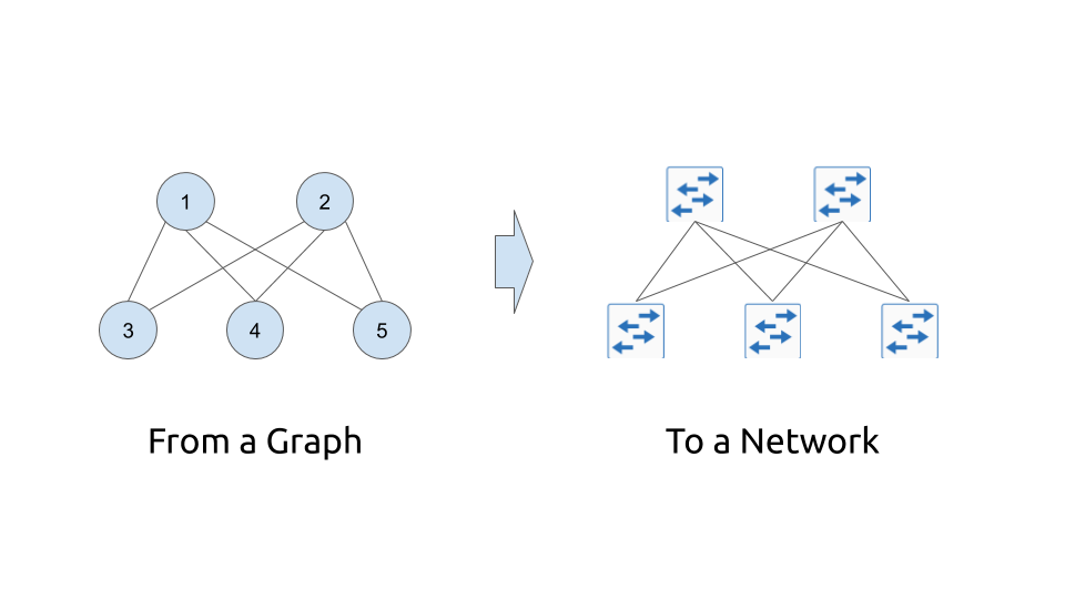
Going back to the questions mentioned above… Abstracting from the burden of the physical infrastructure issues, the network topology is just a graph. In the simplistic form, it is an interconnection of the nodes (network functions) using edges (links between network functions). The nodes are interconnected with each other by edges under certain rules
For data centres:
- The hosts are interconnected with the leafs within the rack.
- All the leafs are interconnected with all the spines within the pod.
- All the spines are interconnected with all (or under some of) the aggregation (or A-Z switches)
For service providers:
- The PE routers are interconnected with P routers inside the region.
- The P routers are connected to each other in a full mesh scenario or following some rules (e.g. partial mesh with some hub sites).
- All the backhaul aggregation routers are connected to back to the PE in the region.
- The access router are connected to the sub-region aggregations.
For enterprises:
- The modern enterprise network would follow the data centre design pretty much with some exceptions.
All in all, the nodes and edges altogether builds the graph of your network.
On top of that you can start adding the complexity in form of the attributes, which can contain any meta data, such as links’ capacity, routers’ IDs, BGP AS numbers and so on.
Having realised this idea I’ve started thinking that it would be cool to create some basic tool which can do some job for you:
- Generate the topology (either the intend or the actual) of your network based on the design rules you have.
- Generate the standard configuration of your network.
- Deploy the network emulation using Docker or KVM including nodes and necessary links.
- Run the connectivity checks or any other tests you might need to do
All the mentioned tasks should be done in the fully automated approach using the minimum necessary input.
In the previous projects, such as the Service Provider Fabric or the Data Centre Fabric I have used mainly Ansible. In this project I will rely on Python predominantly.
Follow our free Python 3.8 classes in the Code EXpress (CEX) blogs.
What are we going to test?
As we are slowly starting with a new series, the today’s focus will be the following:
- Define the design rules for the topology generation.
- Create an input for the topology generation in the easy human-readable format.
- Generate the topology information in form of graph.
- Visualise the graph using open source visualisation tools.
Software version
The lab setup is the same as we used earlier in the Code EXpress (CEX) series. Actually, it it is exactly the same lab.
Management host:
- CentOS 7.7.1908
- Bash 4.2.26
- Python 3.8.2
- Docker-CE 19.03.8
- Graphviz 2.30.1
The hyper scale data centre fabric is not present in the form of the network element today.
The basic design was provided in the previous blogpost about the Microsoft Azure SONiC and Docker. However, that will be changed soon by the automation.
Topology
There is no topology per SE yet, as we will define the design rules and implement them using Python in this article.
If you want to go straight to the code, jump to our GitHub.
Solution development
The outline of the activities we are going to cover today is listed above, so let’s crack on them. But before that, take a look on the diagram of the files structure for this code:
2
3
4
5
6
7
8
| +--build.yml
+--main.py
+--prepare.sh
+--requirements.txt
+--topology
+--autogen.gv
+--autogen.gv.png
The inventory folder contains the file with the physical topology called build.yml. The main.py is a core Python code, we are developing now, whereas the requirements.txt contains the list of the external Python libraries we need to install to make our code working. The prepare.sh Bash script automates the installation of the Graphviz. The topology directory has two files inside, which are (or will be) generated during the execution of our Python’s program.
#1. The rules of the network modelling
Building of the hyper scale data centre is a very interesting topic, as it have some certain differences comparing to the enterprise data centres. The enterprise data centres requires in the vast majority a lot of east-west traffic based on the traditional enterprise applications’ design, whereas the hyper scale data centres build with the requirements of the capacity between the applications and consumers outside of the data centres. Therefore, the scaling requirements are much tougher. As a basis for the design rules we’ll take the ones described in the Facebook engineering blog. Simplifying them a bit, here is the what we are going to implement:
- The network consists of multiple pods.
- Each pod has four spines and four leafs. Each leaf is connected to each spine.
- Each leaf has one host connected.
- There is a data centre aggregation level consisting of four planes. Each plane consists of one aggs.
- Each spine is connected to each aggregation plane; hence, to each aggs.
The number of leafs or spines per pod could be easily increased, as there is no hardcoding done in the Python’s code about that.
These rules described above will be implemented in the Python 3.8 code.
#2. The user input for the hyper scale data centre fabric
The next important point is to identify what we leave for the network developer to provide as an input for this tool. We might limit the input only to the amount of the pods and, perhaps, we will implement that in future. For now we’ll retain more control and will manually create the list of the devices. We don’t need to provide the connectivity between the network fabric functions as they will be automatically generated (we skip the ports naming for now and implement them in a next release). However, we will add the connectivity details for the host as we want to have a determinism here.
We said, we want to provide the input in a human-readable format. Therefore, we will use YAML for that. The input for the data centre build is the following:
2
3
4
5
6
7
8
9
10
11
12
13
14
15
16
17
18
19
20
21
22
23
24
25
26
27
28
29
30
31
32
33
34
35
36
37
38
39
40
41
42
43
44
45
46
47
48
49
50
51
52
53
54
55
56
57
58
59
60
61
62
63
64
65
66
67
68
69
70
71
72
73
74
75
76
77
78
79
80
81
82
83
84
85
86
87
88
89
90
91
92
93
94
95
96
97
98
99
---
aggs:
- name: aggs1
pod:
dev_type: microsoft-sonic
- name: aggs2
pod:
dev_type: microsoft-sonic
- name: aggs3
pod:
dev_type: microsoft-sonic
- name: aggs4
pod:
dev_type: microsoft-sonic
spines:
- name: spine11
pod: A
dev_type: microsoft-sonic
- name: spine12
pod: A
dev_type: microsoft-sonic
- name: spine13
pod: A
dev_type: microsoft-sonic
- name: spine14
pod: A
dev_type: microsoft-sonic
- name: spine21
pod: B
dev_type: microsoft-sonic
- name: spine22
pod: B
dev_type: microsoft-sonic
- name: spine23
pod: B
dev_type: microsoft-sonic
- name: spine24
pod: B
dev_type: microsoft-sonic
leafs:
- name: leaf11
pod: A
dev_type: microsoft-sonic
- name: leaf12
pod: A
dev_type: microsoft-sonic
- name: leaf13
pod: A
dev_type: microsoft-sonic
- name: leaf14
pod: A
dev_type: microsoft-sonic
- name: leaf21
pod: B
dev_type: microsoft-sonic
- name: leaf22
pod: B
dev_type: microsoft-sonic
- name: leaf23
pod: B
dev_type: microsoft-sonic
- name: leaf24
pod: B
dev_type: microsoft-sonic
hosts:
- name: host1
pod: A
dev_type: ubuntu
connection_point: leaf11
- name: host2
pod: A
dev_type: ubuntu
connection_point: leaf12
- name: host3
pod: A
dev_type: ubuntu
connection_point: leaf13
- name: host4
pod: A
dev_type: ubuntu
connection_point: leaf14
- name: host5
pod: B
dev_type: ubuntu
connection_point: leaf21
- name: host6
pod: B
dev_type: ubuntu
connection_point: leaf22
- name: host7
pod: B
dev_type: ubuntu
connection_point: leaf23
- name: host8
pod: B
dev_type: ubuntu
connection_point: leaf24
...
The entry for all the element is the same with the exception of the host, which as a specific entry:
- name is a hostname of the device. It is also a node id in the graph.
- pod is a name of the pod the device belongs to. Could be empty for devices not belonging to the pod, such as aggregation fabric or DCI routers.
- dev_type identifies what type of the operation system the virtual or containerised network function.
- connection_point (host-type specific) points the leaf node, where the host should be connected to.
In the future the rules could be changed, but it is enough for now to start with.
#3. The network topology graph
We are approaching the core part of this blogpost. To create a network topology we will use graphs. The implementation of the graphs we are using will be in the DOT language used by Graphviz. The detailed explanation you can find on the provided link, but at a high level you should know the following points:
- The graph is a collection of the nodes and edges.
- The graph could directed (digraph) or undirected (graph). The directed one is used, when it matters the direction of the communication, whereas the undirected one is used (e.g. hops in the trace route), when only the interdependency of the nodes matter without the direction (link between the network functions).
- Each node must have an id by which it is defined in the graph and may have label, which is used in the graph visualisation, or any other meta data.
- The nodes are interconnected between each other used edges. As explained earlier, the edges can be either directed or undirected depending on the graph’s type.
- Each edge must have two and only two endpoints, which are the nodes it interconnects, and may have label, which is used in the graph visualisation, or any other meta data.
There are several libraries existing in the Python, which can be used for working with the graphs. We will use graphviz, which is a Python realisation of the Graphviz tool.
The full documentation to graphviz Python library you can find here.
In order to utilise this package, as well as in order to able to convert YAML into Python’s dictionary, we need to install them using pip. You can do that by putting all the modules you need into a text file, which is provided as in input for the pip tool:
2
3
4
5
6
7
8
9
10
11
12
13
14
pydot
graphviz
pyyaml
$ python -V
Python 3.8.2
$ pip instal -r requirements.txt
Requirement already satisfied: pydot in ./venv/lib/python3.8/site-packages (from -r requirements.txt (line 1)) (1.4.1)
Requirement already satisfied: graphviz in ./venv/lib/python3.8/site-packages (from -r requirements.txt (line 2)) (0.13.2)
Requirement already satisfied: pyyaml in ./venv/lib/python3.8/site-packages (from -r requirements.txt (line 3)) (5.3.1)
Requirement already satisfied: pyparsing>=2.1.4 in ./venv/lib/python3.8/site-packages (from pydot->-r requirements.txt (line 1)) (2.4.7)
One the installation is complete, we create the following tool in Python 3.8:
2
3
4
5
6
7
8
9
10
11
12
13
14
15
16
17
18
19
20
21
22
23
24
25
26
27
28
29
30
31
32
33
34
35
36
37
38
39
40
41
42
43
44
45
46
47
48
#!/usr/bin/env python
# Modules
from graphviz import Graph
import yaml
# Variables
path_inventory = 'inventory/build.yaml'
path_output = 'topology/autogen.gv'
# User-defined functions
def yaml_dict(file_path):
with open(file_path, 'r') as temp_file:
temp_dict = yaml.load(temp_file.read(), Loader=yaml.Loader)
return temp_dict
# Body
if __name__ == '__main__':
inventory = yaml_dict(path_inventory)
dot = Graph(comment='Data Centre', format='png', node_attr={'color': 'deepskyblue1', 'style': 'filled'})
# Adding the devices
for dev_role, dev_list in inventory.items():
for elem in dev_list:
dot.node(elem['name'], pod=elem['pod'], dev_type=elem['dev_type'])
# Adding the nodes
for le in inventory['leafs']:
for ho in inventory['hosts']:
if ho['connection_point'] == le['name']:
dot.edge(le['name'], ho['name'], type='link_customer')
for sp in inventory['spines']:
for le in inventory['leafs']:
if sp['pod'] == le['pod']:
dot.edge(sp['name'], le['name'], type='link_dc')
for ag in inventory['aggs']:
for sp in inventory['spines']:
dot.edge(ag['name'], sp['name'], type='link_dc')
with open(path_output, 'w') as file:
file.write(dot.source)
Join our network automation training to learn the basics and advanced topics of the network automation development in Python 3.
Step by step the provided Python’s code do the following actions:
- Importing the necessary modules into our Python code.
- Creating the variables with the path to the input (YAML topology) and the output (file with the generated graph).
- Creating the user-defined function, which converts the YAML file into the Python dictionary.
- Importing the YAML topology.
- Creating a Python’s object for a graph using the imported class. There are some parameters are provided, such as a name of the graph in the comment, the format and the node attributes of the visualisation (used later)
- Using the for loops and the if conditionals populate the object with the nodes and links based on the design rules explained above.
- Saves the resulting node in a graph file.
The Python’s object, classes and work with files are not covered yet in the first 10 Code EXpress (CEX) episodes. They will be covered on later in the second saison.
Let’s try to execute the code and see the results:
2
3
4
5
6
7
8
9
10
11
12
13
14
15
16
17
18
19
20
21
22
23
24
25
26
27
28
29
30
31
32
33
34
35
36
37
38
39
40
41
42
43
44
45
46
47
48
49
50
51
52
53
54
55
56
57
58
59
60
61
62
63
64
65
66
67
68
69
70
71
72
73
74
75
76
77
78
79
80
81
82
83
84
85
86
87
88
89
90
91
92
93
94
95
96
97
98
99
100
101
102
103
104
105
106
107
108
$ cat topology/autogen.gv
// Data Centre
graph {
node [color=deepskyblue1 style=filled]
aggs1 [dev_type="microsoft-sonic"]
aggs2 [dev_type="microsoft-sonic"]
aggs3 [dev_type="microsoft-sonic"]
aggs4 [dev_type="microsoft-sonic"]
spine11 [dev_type="microsoft-sonic" pod=A]
spine12 [dev_type="microsoft-sonic" pod=A]
spine13 [dev_type="microsoft-sonic" pod=A]
spine14 [dev_type="microsoft-sonic" pod=A]
spine21 [dev_type="microsoft-sonic" pod=B]
spine22 [dev_type="microsoft-sonic" pod=B]
spine23 [dev_type="microsoft-sonic" pod=B]
spine24 [dev_type="microsoft-sonic" pod=B]
leaf11 [dev_type="microsoft-sonic" pod=A]
leaf12 [dev_type="microsoft-sonic" pod=A]
leaf13 [dev_type="microsoft-sonic" pod=A]
leaf14 [dev_type="microsoft-sonic" pod=A]
leaf21 [dev_type="microsoft-sonic" pod=B]
leaf22 [dev_type="microsoft-sonic" pod=B]
leaf23 [dev_type="microsoft-sonic" pod=B]
leaf24 [dev_type="microsoft-sonic" pod=B]
host1 [dev_type=ubuntu pod=A]
host2 [dev_type=ubuntu pod=A]
host3 [dev_type=ubuntu pod=A]
host4 [dev_type=ubuntu pod=A]
host5 [dev_type=ubuntu pod=A]
host6 [dev_type=ubuntu pod=B]
host7 [dev_type=ubuntu pod=B]
host8 [dev_type=ubuntu pod=B]
leaf11 -- host1 [type=link_customer]
leaf12 -- host2 [type=link_customer]
leaf13 -- host3 [type=link_customer]
leaf14 -- host4 [type=link_customer]
leaf21 -- host5 [type=link_customer]
leaf22 -- host6 [type=link_customer]
leaf23 -- host7 [type=link_customer]
leaf24 -- host8 [type=link_customer]
spine11 -- leaf11 [type=link_dc]
spine11 -- leaf12 [type=link_dc]
spine11 -- leaf13 [type=link_dc]
spine11 -- leaf14 [type=link_dc]
spine12 -- leaf11 [type=link_dc]
spine12 -- leaf12 [type=link_dc]
spine12 -- leaf13 [type=link_dc]
spine12 -- leaf14 [type=link_dc]
spine13 -- leaf11 [type=link_dc]
spine13 -- leaf12 [type=link_dc]
spine13 -- leaf13 [type=link_dc]
spine13 -- leaf14 [type=link_dc]
spine14 -- leaf11 [type=link_dc]
spine14 -- leaf12 [type=link_dc]
spine14 -- leaf13 [type=link_dc]
spine14 -- leaf14 [type=link_dc]
spine21 -- leaf21 [type=link_dc]
spine21 -- leaf22 [type=link_dc]
spine21 -- leaf23 [type=link_dc]
spine21 -- leaf24 [type=link_dc]
spine22 -- leaf21 [type=link_dc]
spine22 -- leaf22 [type=link_dc]
spine22 -- leaf23 [type=link_dc]
spine22 -- leaf24 [type=link_dc]
spine23 -- leaf21 [type=link_dc]
spine23 -- leaf22 [type=link_dc]
spine23 -- leaf23 [type=link_dc]
spine23 -- leaf24 [type=link_dc]
spine24 -- leaf21 [type=link_dc]
spine24 -- leaf22 [type=link_dc]
spine24 -- leaf23 [type=link_dc]
spine24 -- leaf24 [type=link_dc]
aggs1 -- spine11 [type=link_dc]
aggs1 -- spine12 [type=link_dc]
aggs1 -- spine13 [type=link_dc]
aggs1 -- spine14 [type=link_dc]
aggs1 -- spine21 [type=link_dc]
aggs1 -- spine22 [type=link_dc]
aggs1 -- spine23 [type=link_dc]
aggs1 -- spine24 [type=link_dc]
aggs2 -- spine11 [type=link_dc]
aggs2 -- spine12 [type=link_dc]
aggs2 -- spine13 [type=link_dc]
aggs2 -- spine14 [type=link_dc]
aggs2 -- spine21 [type=link_dc]
aggs2 -- spine22 [type=link_dc]
aggs2 -- spine23 [type=link_dc]
aggs2 -- spine24 [type=link_dc]
aggs3 -- spine11 [type=link_dc]
aggs3 -- spine12 [type=link_dc]
aggs3 -- spine13 [type=link_dc]
aggs3 -- spine14 [type=link_dc]
aggs3 -- spine21 [type=link_dc]
aggs3 -- spine22 [type=link_dc]
aggs3 -- spine23 [type=link_dc]
aggs3 -- spine24 [type=link_dc]
aggs4 -- spine11 [type=link_dc]
aggs4 -- spine12 [type=link_dc]
aggs4 -- spine13 [type=link_dc]
aggs4 -- spine14 [type=link_dc]
aggs4 -- spine21 [type=link_dc]
aggs4 -- spine22 [type=link_dc]
aggs4 -- spine23 [type=link_dc]
aggs4 -- spine24 [type=link_dc]
}
This graph provides already a lot of information about our network topology including the meta data we will need future to automatically insatiate our virtual topology. It doesn’t have yet all the necessary details, such as IP addresses, port names and BGP AS numbers, though.
These features would be covered in the next blogpost.
Reading the graph for human beings might be a bit challenging. Therefore, we are moving to the last step in this blogpost.
#4. Visual representation of the network graph.
The Graphviz allows us to generate a nice visual graph in multiple formats. We’ve chosen PNG, as it is easy to use it in any document if we want to describe our network. However, you can save the documents in other formats (e.g. PDF).
In order to create an image, you need to download and install the Graphviz tool to your host. It is an open-source and it has quite a big support of the various platforms. We use CentOS, so we download the necessary RPM and install it as follows:
2
3
4
5
6
7
8
9
10
11
12
#!/usr/bin/env bash
# Download the Graphviz
wget http://rpmfind.net/linux/centos/7.7.1908/os/x86_64/Packages/graphviz-2.30.1-21.el7.x86_64.rpm
# Install the Graphviz
sudo yum localinstall graphviz-2.30.1-21.el7.x86_64.rpm
$ chmod a+x prepare.sh
$ sudo ./prepare.sh
Now we need to add literally one string in our Python code to visualise the DOT graph out of the created file:
2
3
! Information is truncated for brevity
dot.render(path_output, view=True)
By adding a single string we can create with an image of our data centre. Once the script is executed:
2
3
This tool has been deprecated, use 'gio open' instead.
See 'gio help open' for more info
The image is automatically generated and opened:

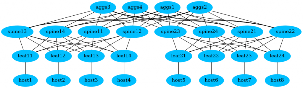
It is already good, but could be a bit better.
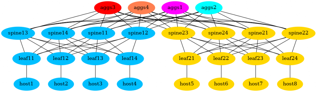
#4.1. Modifying the colours
The data centre consists of the pods. Hence, it would be good to colour the devices from one pod with one colour and the devices from another one with another. Same is applied for the aggregation switches.
To do that, we need to extend our Python’s code. But beforehand, we need to know the names of the colours, which find them in the official documentation to Graphviz.
Knowing the name of the colours, we modify our script in the following way:
2
3
4
5
6
7
8
9
10
11
12
13
14
15
16
17
18
19
20
21
22
23
24
25
26
27
28
29
30
31
32
33
34
35
36
37
38
39
40
41
42
43
44
45
46
47
48
49
50
51
52
53
54
55
#!/usr/bin/env python
# Modules
from graphviz import Graph
import yaml
import random
# Variables
path_inventory = 'inventory/build.yaml'
path_output = 'topology/autogen.gv'
colours = ['deepskyblue', 'gold', 'lightgrey', 'orangered', 'cyan', 'red', 'magenta', 'coral']
chosen_colours = {}
# User-defined functions
def yaml_dict(file_path):
with open(file_path, 'r') as temp_file:
temp_dict = yaml.load(temp_file.read(), Loader=yaml.Loader)
return temp_dict
def set_colour(dev_info, dev_role):
available_colours = len(colours)
colour_choice = 'black'
if dev_role == 'aggs':
colour_choice = colours.pop(random.randrange(available_colours))
chosen_colours[dev_info['name']] = colour_choice
elif dev_info['pod']:
if f'pod_{dev_info["pod"]}' in chosen_colours:
colour_choice = chosen_colours[f'pod_{dev_info["pod"]}']
else:
colour_choice = colours.pop(random.randrange(available_colours))
chosen_colours[f'pod_{dev_info["pod"]}'] = colour_choice
return colour_choice
# Body
if __name__ == '__main__':
inventory = yaml_dict(path_inventory)
dot = Graph(comment='Data Centre', format='png', node_attr={'style': 'filled'})
# Adding the devices
for dev_group, dev_list in inventory.items():
for elem in dev_list:
dot.attr('node', color=set_colour(elem, dev_group))
dot.node(elem['name'], pod=elem['pod'], dev_type=elem['dev_type'])
! Further output is truncated for brevity
In a short words we do the following:
- Creating an empty Python dictionary chosen_colours, which will contain the used colours and the Python list colours with the colours we’d like to use.
- Creating user-defined function set_colour, which allocates the unique colour for each aggregation switch and for each pod.
- Using this function to associate the colour with each node separately.
Once we execute this script once more:
2
3
This tool has been deprecated, use 'gio open' instead.
See 'gio help open' for more info.
We get the same graph, but with the described colour scheme:
GitHub repository
This project is a live one (at lest now). You can find the actual state in our GitHub repository.

Lessons learned
Initially I struggled to build an undirected graph and was able to build only the directed one. However, reading the documentation helped to fix that. As said… RTFM.
Conclusion
The starting of the project is all the time exciting. I have some ideas in my mind to cover up in the some following blogposts as mentioned above. Stay connected and you will see further researches and reflections on building and automating the hyper-scale infrastructure build with its emulation and automated testing. Take care and good bye.
Support us
P.S.
If you have further questions or you need help with your networks, I’m happy to assist you, just send me message. Also don’t forget to share the article on your social media, if you like it.
BR,
Anton Karneliuk