

Hello my friend,
There was quite a considerable amount of the feedbacks on the previous post about the data centre network visualisation with graphs. Originally we planned to cover the topology generation today. However, we changed the plan to improve the math model of our graph to make it more flexible and useful from modelling perspective.
2
3
4
5
retrieval system, or transmitted in any form or by any
means, electronic, mechanical or photocopying, recording,
or otherwise, for commercial purposes without the
prior permission of the author.
Network automation training – boost your career
To be able to understand and, more important, to create such a solutions, you need to have a holistic knowledge about the network automation. Come to our network automation training to get this knowledge and skills.
At this training we teach you all the necessary concepts such as YANG data modelling, working with JSON/YAML/XML data formats, Linux administration basics, programming in Bash/Ansible/Python for multiple network operation systems including Cisco IOS XR, Nokia SR OS, Arista EOS and Cumulus Linux. All the most useful things such as NETCONF, REST API, OpenConfig and many others are there. Don’t miss the opportunity to improve your career.
Thanks
Thanks a lot for all your interactions on the social medias in LinkedIn, Twitter and Facebook. Among others, in particular I’m grateful to:
- Serghei Golipad for inputs on meta-data for graphs
- Lucas Aimaretto for inputs on the NetworkX Python library
- Josh Saul for inputs on the general approach for more detailed graphs and various levels of the abstraction on graphs.
Your inputs and feedbacks helped me to look on some idea, I haven’t though so far in the beginning.
Brief description
The visualisation of the data centre network we did the last time using the Python and Grahviz produced quite a good graphical representation of the information. However, there was a number of the drawbacks:
- The network graph was stored only in DOT language, what made it available for visualisation using Graphviz but not available for analyse in Python.
- The network graph shew the interconnection of the devices without showing further details (e.g. which port was used for connectivity)
- The network graph hasn’t displayed the useful meta data. To be honest, in general the amount of the meta data was tiny.
All these led to the fact that it was impossible to utilise the generated network graph for anything besides the visualisation itself. Therefore, we need to address the mentioned drawbacks before we go further. That’s what we are going to do today.
What are we going to test?
The major focus is to make our network graph available for the math analysis and automated network topology instantiation in Linux:
- Find a way how to manage graph as a set of the objects (nodes and edges) with parameters/attributes.
- Add new nodes’ type, which represent interfaces of the devices.
- Add the data needed to build a topology (IP address, BGP AS numbers).
- Make sure that the new graph is visualised properly using Graphviz as we used before.
Software version
So far in this series, the core technology for us is Python. The lab setup for Python 3.8 was covered the Code EXpress (CEX) series. Hence, we are reusing the same setup.
The network automation development host runs the following toolkit:
- CentOS 7.7.1908
- Bash 4.2.26
- Python 3.8.2
- Docker-CE 19.03.8
- Graphviz 2.30.1
- NetworkX 2.4
The basic design was provided in the previous blogpost about the Microsoft Azure SONiC and Docker. However, that will be changed soon by the automation.
Topology
The design rules for the hyper-scale data centre network were provided in the previous post. Based on those rules we have implemented the first generation of the network graph showing the network nodes:

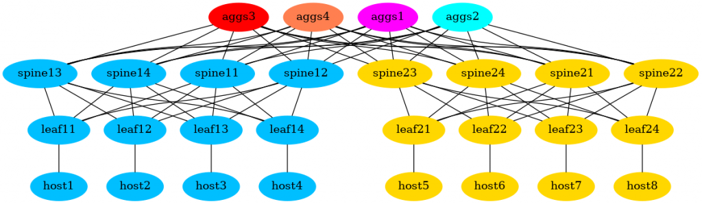
Today this graph will be significantly improved, but it will retain the same logic and connectivity rules.
You can take a look at the code in our GitHub repository.
Solution development
We will be addressing the issues in the stepwise approach, one problem at a time. And we start with the modification of the graphs.
#1. Graph as at of objects
So we want to make network graph a real graph, with nodes and edges having attributes. By doing so we mean the possibility to have these attributes available in Python for processing.
After some investigations we’ve found a brilliant Python’s package for the graphs, which fulfils our requirements. It is called NetworkX. Per the description from the website:
NetworkX is a Python package for the creation, manipulation, and study of the structure, dynamics, and functions of complex networks
https://networkx.github.io
Is a hyper-scale data centre network complex and dynamic enough? 🙂 We thought so and tried to use this package. The results are quite impressive, but we have to rewrite the Python’s code completely. This is entirely fine as we are just in the beginning of our project, so the changes are easy to adopt.
The documentation of the NetworkX Python’s package is very extensive; therefore, we managed to rewrite our code following the original logic:
- Adding the nodes with the attributes
- Adding the edges between the nodes with the attributes
At a high level, the following syntax is used to work with graphs in NetworkX:
2
3
4
5
6
7
8
9
10
import networkx
DG = networkx.Graph(label='Data Centre')
DG.add_node(node1, meta1=val, meta2=val, .., metaN=val)
DG.add_node(node2, meta1=val, meta2=val, .., metaN=val)
DG.add_edge(node1, node2, meta1=val, meta2=val, .., metaN=val)
Using such a syntax we create a math model of the graph, which is not related to the Graphviz. However, later on we will use the Graphviz tool we already used earlier to visualise the graph created NetworkX.
The reason why we are so passionate about the NetworkX is that it allows us to call each element and get it metadata. For example, calling the graph in such a way:
2
>>> {'pod': 'A', 'dev_type': 'microsoft-sonic', 'dev_role': 'leafs', 'style': 'filled', 'fillcolor': 'magenta', 'rank': 7, 'bgp_asn': 65012, 'label': 'leaf11\n65012\n10.0.255.12', 'loopback': '10.0.255.12'}
returns the Python’s dictionary with all the metadata associated with the object. Same is true for the edges:
2
>>> {'phy': 'wire', 'role': 'customer', 'color': 'coral', 'linux_bridge': 'hs_br_0'}
where this would return the meta data associated with the edge.
Therefore, using the NetworkX the network graph for our hyper-scale data centre is a real graph and we can move to the next topic, we need to revise.
#2. Grahpviz for visualisation of NetworkX graphs
More precisely, we move to the visualisation of the network graph. The last time we have used Grahpviz tool and graphviz Python’s package. This time we continue using the Graphviz tool, but instead of the latter we will use pygraphviz package. This Python’s package provides the interfaces for the NetworkX to use the Graphviz. Hence, we can benefit from the both worlds: working with the graph and do the math analysis and modelling using NetworkX and create a visualisation using the DOT language using Graphviz.
The NetworkX already has an integration with pygraphviz internally. Hence, the only thing we need is to install that package into our virtual environment and make sure that we call the proper classes in the NetworkX:
2
3
4
5
6
7
8
import networkx
DG = networkx.Graph(label='Data Centre')
VG = networkx.drawing.nx_agraph.to_agraph(DG)
VG.layout('dot')
VG.draw('output.png')
Once we rewrite the code with the NetworkX and pygraphviz and try to regenerate the graph, we come exactly to the same result as we have shown above:
What confirms the point the visualisation stays consistent, despite we have changed the internal structure of our graph.
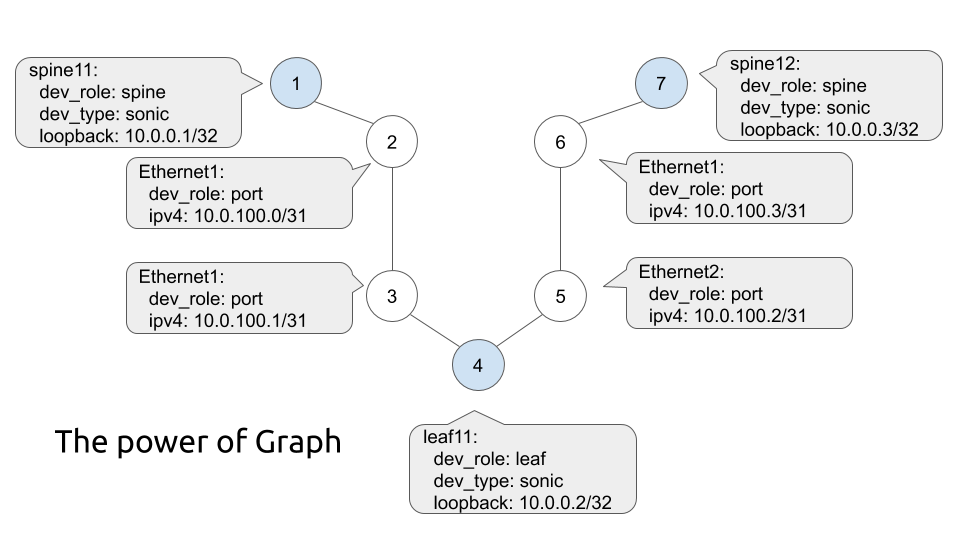
#3. Adding new nodes and missing meta data for nodes and edges
Our initial graph didn’t have any information about the following items:
- physical interfaces, which devices use to connect to each other.
- IP addresses associated with these interfaces or with the the loopback interfaces.
- BGP AS numbers associated with the leafs, spines and aggregation spines.
As this information is critical for the modelling of the real network, its absence made impossible the automated network emulation in Linux. The solution we decided to implement is the following:
- Create a file with resources, which list the base IP addresses for the loopbacks, point-to-point data centre interfaces and customer connections, and BGP AS numbers
- Using Python’s packages called netaddr made a necessary adjustments of the base IP addresses to create a unique IP address per interface.
- Allocate the unique BGP AS number for each spine, leaf and aggregation spine.
The file with the base resources is placed in the inventory directory, where we already have build.yaml:
2
3
4
5
6
7
8
9
10
---
bgp:
asn: 65000
ip:
loop: 10.0.255.0/24
dc: 10.0.0.0/24
customer: 192.168.10.0/24
...
The part of the code, which generates the BGP ASN and IP addresses for the loopbacks is integrated into the process of building the network graph (adding nodes, to be precise):
2
3
4
5
6
7
8
9
10
11
12
13
14
15
16
17
18
19
20
21
22
23
DG = networkx.Graph(label='Data Centre')
# Adding the devices to the graph
dev_id = 0
ip_addr = netaddr.IPNetwork(resources['ip']['loop'])
for dev_group, dev_list in inventory.items():
for elem in dev_list:
DG.add_node(elem['name'], pod=elem['pod'],
dev_type=elem['dev_type'], dev_role=dev_group,
style='filled', fillcolor=set_colour(elem, dev_group),
rank=set_rank(resources['ranks'], [dev_group, None]))
if dev_group in ['aggs', 'spines', 'leafs']:
DG.nodes[elem['name']]['bgp_asn'] = resources['bgp']['asn'] + dev_id
DG.nodes[elem['name']]['label'] = f'{elem["name"]}\n{resources["bgp"]["asn"] + dev_id}\n{ip_addr[dev_id]}'
DG.nodes[elem['name']]['loopback'] = str(ip_addr[dev_id])
dev_id += 1
list_of_primitives.append(elem['dev_type']) if elem['dev_type'] not in list_of_primitives else None
if_count[elem['name']] = 0
Basically, here we do the following:
- Creating the undirected graph using the networkx class Graph.
- Creating the device counter dev_id, which is counting the number of the network elements in the data centre fabric (excluding customers’ hosts).
- Using netaddr module create a specific object with IP address.
- Adding nodes and their attributes to the graph using for loop control.
- Using if statement code flow control adding some node’s attributes only to the network functions.
There is one more step, we are doing in the provided snippet. We create a Python list called list_of_primitives to collect all the devices’ types we have in the network. This list is used later import the primitives, containing the naming convention for the interfaces and so on per device type:
2
3
4
5
6
7
8
9
10
11
12
13
---
iface:
name: Ethernet
start: 0
...
$ cat primitives/ubuntu.yaml
---
iface:
name: eth
start: 0
...
The content of these files are imported into the main Python’s code and used to generate the new nodes, which have dev_type=port:
2
3
4
5
6
7
8
9
10
11
12
13
14
15
16
17
18
19
20
21
22
23
24
25
26
27
primitives = {}
for primitve_entry in list_of_primitives:
primitives[primitve_entry] = yaml_dict(f'{path_primitives}/{primitve_entry}.yaml')
# Adding the links to the graph
if_id = 0
ip_addr = netaddr.IPNetwork(resources['ip']['customer'])
for le in inventory['leafs']:
for ho in inventory['hosts']:
if ho['connection_point'] == le['name']:
DG.add_node(f'iface-{if_id}', label=f'{primitives[le["dev_type"]]["iface"]["name"]}{if_count[le["name"]]}\n{str(ip_addr[if_id]).split("/")[0]}/31',
ipv4=f'{str(ip_addr[if_id]).split("/")[0]}/31',
dev_type='port', rank=set_rank(resources['ranks'], [DG.nodes[le["name"]]["dev_role"], DG.nodes[ho["name"]]["dev_role"]]))
DG.add_edge(le['name'], f'iface-{if_id}', phy='port', color='black')
DG.add_node(f'iface-{if_id + 1}', label=f'{primitives[ho["dev_type"]]["iface"]["name"]}{if_count[ho["name"]]}\n{str(ip_addr[if_id + 1]).split("/")[0]}/31',
ipv4=f'{str(ip_addr[if_id + 1]).split("/")[0]}/31',
dev_type='port', rank=set_rank(resources['ranks'], [DG.nodes[ho["name"]]["dev_role"], DG.nodes[le["name"]]["dev_role"]]))
DG.add_edge(ho['name'], f'iface-{if_id + 1}', phy='port', color='black')
DG.add_edge(f'iface-{if_id}', f'iface-{if_id + 1}', phy='wire', role='customer', color='coral', linux_bridge=f'hs_br_{if_id}')
if_id += 2
if_count[le["name"]] += 1
if_count[ho["name"]] += 1
The conversion of the YAML file into a Python dictionary was explained in the previous blog.
The core idea in the code above to add the following elements to the existing graph:
- Add node with the dev_type=port and the name out of the primitives of the first node for this link, as well as IP address out of the listed resources as an attribute.
- Add edge between the created node and this first node.
- Add node with the dev_type=port and the name out of the primitives of the second node for this link, as well as IP address out of the listed resourcesas an attribute.
- Add edge between the created node and this second node.
- Add edge between two created port nodes and add the attribute of the link type, as well as the attribute linux_bridge, which is unique per link and will be used in future to automatically generate the Linux bridges for the network emulation.
The code might looks complex. However, if you carefully reviews it, you can understand it as the logic is pretty straightforward.
#4. Moving user-defined functions out of the main Python’s script
The last step before showing you the results of the Python’s code modification is the move of the part of the code, which contains all the user-defined functions we’ve created in the previous and current steps into a separate file called localfunctions.py, which we put into the directory bin:
2
3
4
5
6
7
8
9
10
11
12
13
14
15
16
17
18
19
20
21
22
23
24
25
26
27
28
29
30
31
32
33
34
35
36
37
38
39
40
41
42
43
44
45
46
#!/usr/bin/env python
# Modules
import yaml
import random
# Variables
colours = ['deepskyblue', 'gold', 'lightgrey', 'orangered', 'cyan', 'red', 'magenta', 'coral']
chosen_colours = {}
# User-defined functions
def yaml_dict(file_path):
with open(file_path, 'r') as temp_file:
temp_dict = yaml.load(temp_file.read(), Loader=yaml.Loader)
return temp_dict
def set_colour(dev_info, dev_role):
available_colours = len(colours)
colour_choice = 'black'
if dev_role == 'aggs':
colour_choice = colours.pop(random.randrange(available_colours))
chosen_colours[dev_info['name']] = colour_choice
elif dev_info['pod']:
if f'pod_{dev_info["pod"]}' in chosen_colours:
colour_choice = chosen_colours[f'pod_{dev_info["pod"]}']
else:
colour_choice = colours.pop(random.randrange(available_colours))
chosen_colours[f'pod_{dev_info["pod"]}'] = colour_choice
return colour_choice
def set_rank(build_res, list_nodes):
if not list_nodes[1]:
r = build_res[f'{list_nodes[0]}']
else:
r = build_res[f'if_{list_nodes[0]}_{list_nodes[1]}']
return r
Such a move allows us to limit the size of the main program and split the main logic from the supporting functions, even if they are very important.
In future we might also move the network graph build into a separate file, but it is not yet the case.
#5. Putting all together
You might feel a bit confused watching various pieces of the Python code, if you haven’t read the previous blogpost. Even if you have read, it might be a bit challenging. The modified architecture of the directory with the project looks like as follows:
2
3
4
5
6
7
8
9
10
11
12
13
14
| +--localfunctions.py
+--inventory
| +--build.yaml
| +--resources.yaml
+--main.py
+--prepare.sh
+--primitives
| +--microsoft-sonic.yaml
| +--ubuntu.yaml
+--requirements.txt
+--topology
+--autogen.gv
+--autogen.gv.png
You have also seen all new files together with the explanation what are they aim to solve. Now we will show you the final main.py, which is a core Python’s code in this project:
2
3
4
5
6
7
8
9
10
11
12
13
14
15
16
17
18
19
20
21
22
23
24
25
26
27
28
29
30
31
32
33
34
35
36
37
38
39
40
41
42
43
44
45
46
47
48
49
50
51
52
53
54
55
56
57
58
59
60
61
62
63
64
65
66
67
68
69
70
71
72
73
74
75
76
77
78
79
80
81
82
83
84
85
86
87
88
89
90
91
92
93
94
95
96
97
98
99
100
101
102
103
104
105
106
107
108
109
110
111
112
113
114
115
116
117
118
119
120
121
122
123
# Modules
from bin.localfunctions import *
import networkx
import netaddr
# Variables
path_inventory = 'inventory/build.yaml'
parh_resources = 'inventory/resources.yaml'
path_output = 'topology/autogen.gv'
path_primitives = 'primitives'
list_of_primitives = []
if_count = {}
# Body
if __name__ == '__main__':
# Loading resources
inventory = yaml_dict(path_inventory)
resources = yaml_dict(parh_resources)
# Creating graph
DG = networkx.Graph(label='Data Centre')
# Adding the devices to the graph
dev_id = 0
ip_addr = netaddr.IPNetwork(resources['ip']['loop'])
for dev_group, dev_list in inventory.items():
for elem in dev_list:
DG.add_node(elem['name'], pod=elem['pod'],
dev_type=elem['dev_type'], dev_role=dev_group,
style='filled', fillcolor=set_colour(elem, dev_group),
rank=set_rank(resources['ranks'], [dev_group, None]))
if dev_group in ['aggs', 'spines', 'leafs']:
DG.nodes[elem['name']]['bgp_asn'] = resources['bgp']['asn'] + dev_id
DG.nodes[elem['name']]['label'] = f'{elem["name"]}\n{resources["bgp"]["asn"] + dev_id}\n{ip_addr[dev_id]}'
DG.nodes[elem['name']]['loopback'] = str(ip_addr[dev_id])
dev_id += 1
list_of_primitives.append(elem['dev_type']) if elem['dev_type'] not in list_of_primitives else None
if_count[elem['name']] = 0
# Loading the primitives
primitives = {}
for primitve_entry in list_of_primitives:
primitives[primitve_entry] = yaml_dict(f'{path_primitives}/{primitve_entry}.yaml')
# Adding the links to the graph
if_id = 0
ip_addr = netaddr.IPNetwork(resources['ip']['customer'])
for le in inventory['leafs']:
for ho in inventory['hosts']:
if ho['connection_point'] == le['name']:
DG.add_node(f'iface-{if_id}', label=f'{primitives[le["dev_type"]]["iface"]["name"]}{if_count[le["name"]]}\n{str(ip_addr[if_id]).split("/")[0]}/31',
ipv4=f'{str(ip_addr[if_id]).split("/")[0]}/31',
dev_type='port', rank=set_rank(resources['ranks'], [DG.nodes[le["name"]]["dev_role"], DG.nodes[ho["name"]]["dev_role"]]))
DG.add_edge(le['name'], f'iface-{if_id}', phy='port', color='black')
DG.add_node(f'iface-{if_id + 1}', label=f'{primitives[ho["dev_type"]]["iface"]["name"]}{if_count[ho["name"]]}\n{str(ip_addr[if_id + 1]).split("/")[0]}/31',
ipv4=f'{str(ip_addr[if_id + 1]).split("/")[0]}/31',
dev_type='port', rank=set_rank(resources['ranks'], [DG.nodes[ho["name"]]["dev_role"], DG.nodes[le["name"]]["dev_role"]]))
DG.add_edge(ho['name'], f'iface-{if_id + 1}', phy='port', color='black')
DG.add_edge(f'iface-{if_id}', f'iface-{if_id + 1}', phy='wire', role='customer', color='coral', linux_bridge=f'hs_br_{if_id}')
if_id += 2
if_count[le["name"]] += 1
if_count[ho["name"]] += 1
ip_addr = netaddr.IPNetwork(resources['ip']['dc'])
for sp in inventory['spines']:
for le in inventory['leafs']:
if sp['pod'] == le['pod']:
DG.add_node(f'iface-{if_id}', label=f'{primitives[sp["dev_type"]]["iface"]["name"]}{if_count[sp["name"]]}\n{str(ip_addr[if_id]).split("/")[0]}/31',
ipv4=f'{str(ip_addr[if_id]).split("/")[0]}/31',
dev_type='port', rank=set_rank(resources['ranks'], [DG.nodes[sp["name"]]["dev_role"], DG.nodes[le["name"]]["dev_role"]]))
DG.add_edge(sp['name'], f'iface-{if_id}', phy='port', color='black')
DG.add_node(f'iface-{if_id + 1}', label=f'{primitives[le["dev_type"]]["iface"]["name"]}{if_count[le["name"]]}\n{str(ip_addr[if_id + 1]).split("/")[0]}/31',
ipv4=f'{str(ip_addr[if_id + 1]).split("/")[0]}/31',
dev_type='port', rank=set_rank(resources['ranks'], [DG.nodes[le["name"]]["dev_role"], DG.nodes[sp["name"]]["dev_role"]]))
DG.add_edge(le['name'], f'iface-{if_id + 1}', phy='port', color='black')
DG.add_edge(f'iface-{if_id}', f'iface-{if_id + 1}', phy='wire', role='dc', color='coral', linux_bridge=f'hs_br_{if_id}')
if_id += 2
if_count[sp["name"]] += 1
if_count[le["name"]] += 1
for ag in inventory['aggs']:
for sp in inventory['spines']:
DG.add_node(f'iface-{if_id}', label=f'{primitives[ag["dev_type"]]["iface"]["name"]}{if_count[ag["name"]]}\n{str(ip_addr[if_id]).split("/")[0]}/31',
ipv4=f'{str(ip_addr[if_id]).split("/")[0]}/31',
dev_type='port', rank=set_rank(resources['ranks'], [DG.nodes[ag["name"]]["dev_role"], DG.nodes[sp["name"]]["dev_role"]]))
DG.add_edge(ag['name'], f'iface-{if_id}', phy='port', color='black')
DG.add_node(f'iface-{if_id + 1}', label=f'{primitives[sp["dev_type"]]["iface"]["name"]}{if_count[sp["name"]]}\n{str(ip_addr[if_id + 1]).split("/")[0]}/31',
ipv4=f'{str(ip_addr[if_id + 1]).split("/")[0]}/31',
dev_type='port', rank=set_rank(resources['ranks'], [DG.nodes[sp["name"]]["dev_role"], DG.nodes[ag["name"]]["dev_role"]]))
DG.add_edge(sp['name'], f'iface-{if_id + 1}', phy='port', color='black')
DG.add_edge(f'iface-{if_id}', f'iface-{if_id + 1}', phy='wire', role='dc', color='coral', linux_bridge=f'hs_br_{if_id}')
if_id += 2
if_count[ag["name"]] += 1
if_count[sp["name"]] += 1
# Visualising the graph
VG = networkx.drawing.nx_agraph.to_agraph(DG)
with open(path_output, 'w') as file:
file.write(str(VG))
VG.layout('dot')
VG.draw(f'{path_output}.png')
Netaddr is not a built-in module. Therefore, you need to add it to the requirements.txt and install it via pip.
During the execution all the data is stored in the graph DG, which behaves as explained above. The result of the script execution so far is the same: it prints the network graph. The graph though now is much bigger due to all additional interfaces and links connecting interfaces to the devices and between each other. Let’s take a look:
And check how does the result look like:

The resulting graph’s visualisation is huge. It may look not super nice, but it has a much greater level of the details, comparing the one you’ve seen above. However, from the topology perspective and the data centre building rules, it produces the same high-level outcome.
GitHub repository
This project has evolved since the last week. Stay tuned with the updates in our GitHub repository.


Lessons learned
The key lesson we’ve made is that sometimes it is worth to rebuild everything from scratches, if you see that it makes sense. Start with the Graphviz was a successful one from the standpoint of the visualisation. However, as it prevents us from the further development, we have limit it functionality to pure visualisation moving the graph build and processing to the NetworkX. Now we feel us much better to reach the goal we want.
Conclusion
In this blog we have done a significant step further to improve the modelling approach to the network. Now we can managed the network as a graph accessing the attributes of the devices, interfaces, and links. In the next step we will try to created automated network rollout using the configuration explained in the first article in this series. Take care and good bye.
Support us
P.S.
If you have further questions or you need help with your networks, I’m happy to assist you, just send me message. Also don’t forget to share the article on your social media, if you like it.
BR,
Anton Karneliuk